1/19/23 1/19/23

Object Detection Using YOLOv5 Tutorial – Part 3

Very exciting, you're made it to the 3rd and final part of bus detection with YOLOv5 tutorial. If you haven't been following along this whole time; you can read about the camera setup, data collection and annotation process here. The 2nd part of the tutorial focused on getting the data out of Roboflow, creating a CometML data artifact and training the model. That 2rd article is here.

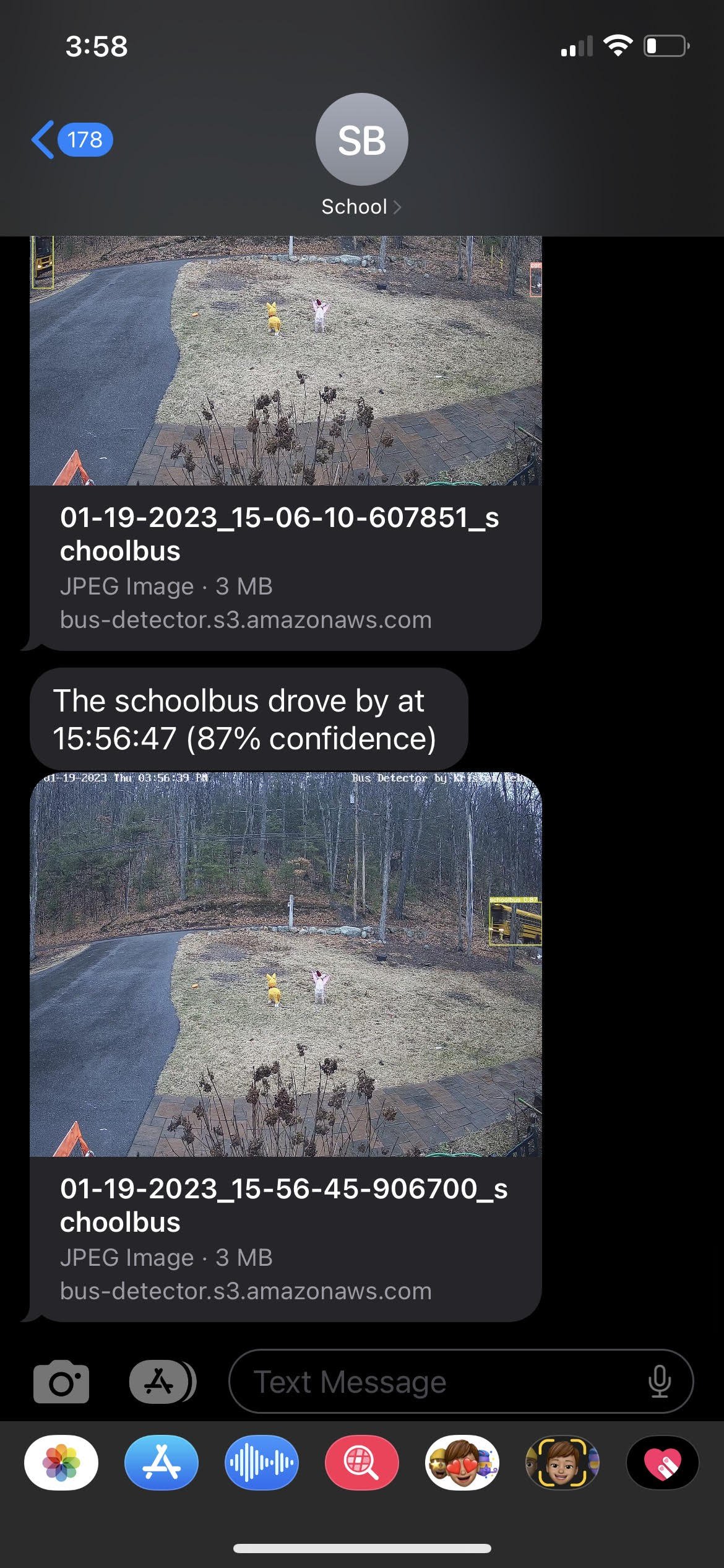
In this article, we're going to take the trained model and actually start doing live detection. Once we detect the bus we'll recieve a text. Here's the steps we're going to go through to set that up:

Choose the best training run
Run live detection
Send a text using AWS

Before we get started, if you’ve tried Coursera or other MOOCs to learn python and you’re still looking for the course that’ll take you much further, like working in VS Code, setting up your environment, and learning through realistic projects.. this is the course I used: Python Course.

Choosing the best training run:

Here we're obviously going to be using Comet. For this project, there were a couple considerations. When I started with too few images there was more value in picking the right model, currently it looks like any of my models trained on the larger set of images would work just fine. Basically, I wanted to minimize false positives, I definitely did not want a text when a neighbor was driving by, because these texts are going to my phone everyday, and that would be annoying. Similarly, it's not a big deal if my model misses classifying a couple frames of the bus, as long as it's catching the bus driving past my house consistently (which consists of a number of frames while driving by my house). We want our precision to be very close to 1.

Run live detection:

It's showtime, folks! For the detection, I forked the YOLOv5 detect script. A link to my copy is here. I need to be able to run my own python code each time the model detects the schoolbus. There are many convenient output formats provided by the yolov5 detect.py script, but for this project I decided to add an additional parameter to the script called "on_objects_detected". This parameter is a reference to a function, and I altered detect.py to call the function whenever it detects objects in the stream. When it calls the function, it also provides a list of detected objects and the annotated image. With this in place, I can define my own function which sends a text message alert and pass that function name to the yolov5 detect script in order to connect the model to my AWS notification code. You can 'CRTL + F' my name 'Kristen' to see the places where I added lines of code and comments.

Sending a text alert:

This was actually my first time using AWS, I had to set up a new account. This Medium article explains how you can set up an AWS account (but not the Go SDK part, I know nothing about Go), but I then used the boto3 library to send the sms.

import os

os.environ['AWS_SHARED_CREDENTIALS_FILE'] = '.aws_credentials'

import boto3


def test_aws_access() -> bool:
    """
    We only try to use aws on detection, so I call this on startup of detect_bus.py to make sure credentials
    are working and everything.  I got sick of having the AWS code fail hours after starting up detect_bus.py...
    I googled how to check if boto3 is authenticated, and found this:
    https://boto3.amazonaws.com/v1/documentation/api/latest/reference/services/sts.html#STS.Client.get_caller_identity
    """
    try:
        resp = boto3.client('sts').get_caller_identity()
        print(f'AWS credentials working.')
        return True
    except Exception as e:
        print(f'Failed to validate AWS authentication: {e}')
        return False


def send_sms(msg):
    boto3.client('sns').publish(
        TopicArn='arn:aws:sns:us-east-1:916437080264:detect_bus',
        Message=msg,
        Subject='bus detector',
        MessageStructure='string')


def save_file(file_path, content_type='image/jpeg'):
    """Save a file to our s3 bucket (file storage in AWS) because we wanted to include an image in the text"""
    client = boto3.client('s3')
    client.upload_file(file_path, 'bus-detector', file_path,
                       ExtraArgs={'ACL': 'public-read', 'ContentType': content_type})
    return f'https://bus-detector.s3.amazonaws.com/{file_path}'

Since we're passing the photo here, you'll get to see the detected picture in the text you receive (below). I went out of my way to add this because I wanted to see what was detected. If it was not a picture of a bus for some reason, I'd like to know what it was actually detecting. Having this information could help inform what type of training data I should add if it wasn't working well.

I also added logic so that I was only notified of the bus once every minute, I certainly don't need a text for each frame of the bus in front of my house. Luckily, it's been working very well. I haven't missed a bus. I have had a couple false positives, but they haven't been in the morning and it's a rare issue.

In order to be allowed to send text messages through AWS SNS in the US, I'm required to have a toll-free number which is registered and verified (AWS docs). Luckily, AWS can provide me with a toll-free number of my own for $2/month. I then used the AWS console to complete the simple TFN registration process where I described the bus detector application and how only my family would be receiving messages from the number (AWS wants to make sure you're not spamming phone numbers).

Getting a .csv of the data:

Although this wasn't part of the intended use case, I'd like to put the bus data over time into a .csv so that I could make a dashboard (really I'm thinking about future projects here, it's not necessary for this project). I've started looking at plots of my data to understand the average time that the bus comes for each of it's passes by my house. I'm starting to see how I could potentially use computer vision and text alerts for other use cases where this data might be more relevant.

import pytz
import boto3
import os

os.environ['AWS_SHARED_CREDENTIALS_FILE'] = '.aws_credentials'

resp = boto3.client('s3').list_objects_v2(
    Bucket='bus-detector',
    Prefix='images/'
)


def get_row_from_s3_img(img):
    local = img['LastModified'].astimezone(pytz.timezone('America/New_York'))
    return {
        'timestamp': local.isoformat(),
        'img_url': f'https://bus-detector.s3.amazonaws.com/{img["Key"]}',
        'class': img['Key'].split('_')[-1].split('.')[0]
    }


images = resp['Contents']
images.sort(reverse=True, key=lambda e: e['LastModified'])
rows = list(map(get_row_from_s3_img, images))

lines = ['timestamp,image_url,class']
for row in rows:
    lines.append(f'{row["timestamp"]},{row["img_url"]},{row["class"]}')

file = open('data.csv', 'w')
file.write('n'.join(lines) + 'n')

Summary:

Well that's it folks. You've been with me on a journey through my computer vision project to detect the school bus. I hope something here can be applied in your own project. In this article we actually ran the detection and set up text alerts, super cool. Through going through this exercise, I can see a number of other ways I could make my life easier using similar technology. Again, the first article about camera setup, data collection, and annotation in Roboflow is here. The 2nd part of the tutorial focused on downloading the data, creating a CometML data artifact and training the model here.

If you’ve tried Coursera or other MOOCs to learn python and you’re still looking for the course that’ll take you much further, like working in VS Code, setting up your environment, and learning through realistic projects.. this is the course I would recommend: Python Course.

10/10/22 10/10/22

Object Detection Using YOLOv5 Tutorial

Welcome! I’ve written this overview of my computer vision project to detect the school bus passing my house. This is for the person who wants to start playing with computer vision and wants to see a project from end-to-end. In this article I’ll start with explaining the problem I’m trying to solve, mention the camera I chose, show a quick opencv tutorial, create images and discuss the different python packages I'm using. The github repo to the project is here. This project will be covered as series of a couple blog posts to get through explaining the rest of the project, so be on the lookout for the next article! The next article will be a guest blog on Roboflow and I'll be sure to link it here.

In this article we’ll cover:

What I’m solving
The libraries I’m using
Setting up the camera
Creating images
Data collection process

The problem:

I wanted to set up a camera and use a computer vision model to detect the school bus when it is passing our house and alert me by sending a text message once the bus is detected. The school bus passes by our house, picks up someone else, and then turns around and then stops at the end of our driveway. This gives us a couple minutes to get my kids ready and out the door once alerted. And now I don’t have to wonder whether or not we’ve missed the bus go by.

The Libraries:

For this project I'm using a number of libraries. Here's a high-level overview of what we'll be working with throughout the project:

yolov5 - This is the object detection model where we will custom train a yolov5 model on our own data. From their repo readme: "YOLOv5 is a family of object detection architectures and models pretrained on the COCO dataset, and represents Ultralytics open-source research into future vision AI methods, incorporating lessons learned and best practices evolved over thousands of hours of research and development."
Roboflow - Loved this GUI for annotating and augmenting the image data that is then be used to train our yolov5 model. Roboflow is an end-to-end CV platform and a library which also provides a Python SDK.
CometML – Comet allows you to basically take a snapshot of your code, dependencies, and anything else needed for your work to be reproducible. With one function you can compare all of your training runs very easily, it’ll even push your runs up to Github for you.
opencv - We're using opencv to access the camera.

Setting up the camera:

I wanted to share about the actual camera I used because finding an appropriate camera wasn’t overly intuitive. I knew that I'd need a friendly api that would work with opencv in python and there was a bit of research before I felt confident the camera would work for my purposes. I went with the ANNKE C500 5MP PoE IP Turret Security Camera it was $60.

opencv can connect to an RTSP compliant security camera (RTSP stands for Real Time Streaming Protocol.. Real time is what we want, baby!). Once we have that setup, we’ll start thinking about collecting our data and then annotating that data using Roboflow.

The instructions for setting up this particular camera were pretty straightforward, I just followed the camera's "getting started" instructions.

Then enter your RTSP address from the camera as your network URL.

Keep that URL handy, you’ll be using that in a couple of places during this project.

The very first step I took once having my camera setup was just to look at the example code in the opencv documentation (cv2) to make sure that things were running. So basically we're going to use VLC to see ourselves on camera and just check that it's all actually working. This is taken directly from the opencv documentation and I only changed the first line of code so that it would use my RTSP URL. I don't have the following code in the repo because it's really just testing and not part of the project.

import numpy as np
import cv2 as cv
cap = cv.VideoCapture("my RTSP URL")
if not cap.isOpened():
    print("Cannot open camera")
    exit()
while True:
    # Capture frame-by-frame
    ret, frame = cap.read()
    # if frame is read correctly ret is True
    if not ret:
        print("Can't receive frame (stream end?). Exiting ...")
        break
    # Our operations on the frame come here
    gray = cv.cvtColor(frame, cv.COLOR_BGR2GRAY)
    # Display the resulting frame
    cv.imshow('frame', gray)
    if cv.waitKey(1) == ord('q'):
        break
# When everything done, release the capture
cap.release()
cv.destroyAllWindows()

After I got to see myself on camera, the next thing I did was set up handling the credentials. This was just to keep my credentials out of version control by saving them in the .camera_credentials file which is excluded from version control with .gitignore. This script takes my credentials and creates the RTSP URL from them. When you call 'detect' in yolov5, the way you do that is by giving it the RTSP URL, so I define a function here called get_rtsp_url().

from os.path import exists
import cv2


def get_rtsp_url():

    # we get the IP address of the camera from our router software
    camera_address = "192.168.4.81"

    # This path and port is documented in our security camera's user manual
    rtsp_path = "/H264/ch1/main/av_stream"
    rtsp_port = 554

    # The name of a file which we will exclude from version control, and save our username and password in it.
    creds_file = '.camera_credentials'

    if not exists(creds_file):
        raise f'Missing configuration file: {creds_file}'

    # This variable will hold the username and password used to connect to
    # the security camera.  Will look like: "username:password"
    camera_auth = open(creds_file, 'r').read().strip()  # open() is how you can read/write files

    # return the open cv object with the authenticated RTSP address.
    full_url = f'rtsp://{camera_auth}@{camera_address}:{rtsp_port}{rtsp_path}'
    return full_url

Next is the connecting_to_camera.py. In a while loop, we're asking for the next frame from the camera and then we save it to the images directory. I also have this create a new directory for each day and for each hour. This made it easier to find and keep track of images easier for me. This is adapted from the opencv documentation.

import numpy as np
import cv2 as cv
from camera import connect_camera
from datetime import datetime
import time
from pathlib import Path
import os

cap = connect_camera()
if not cap.isOpened():
    exit()

img_dir = Path('./school_bus_images/')

while True:
    ret, frame = cap.read()
    if not ret:
        print("Can't receive frame (stream end?). Exiting ...")
        break
    ###  resizing so it won't be so huge
    frame = cv.resize(frame, (int(frame.shape[1] * .5), int(frame.shape[0] * .5)))
    now = datetime.now()

    filename = now.strftime("%m-%d-%Y_%H-%M-%S-%f") + ".jpg"
    day = now.strftime("%m-%d-%Y")
    hour = now.strftime("%H")
    filepath = img_dir / day / hour / filename
    if not (img_dir / day).exists():
        os.mkdir(img_dir / day)
    if not (img_dir / day / hour).exists():
        os.mkdir(img_dir / day / hour)

    cv.imwrite(str(filepath), frame)
    #cv.imshow('frame', frame)
    time.sleep(0.1)



# When everything done, release the capture
cap.release()
cv.destroyAllWindows()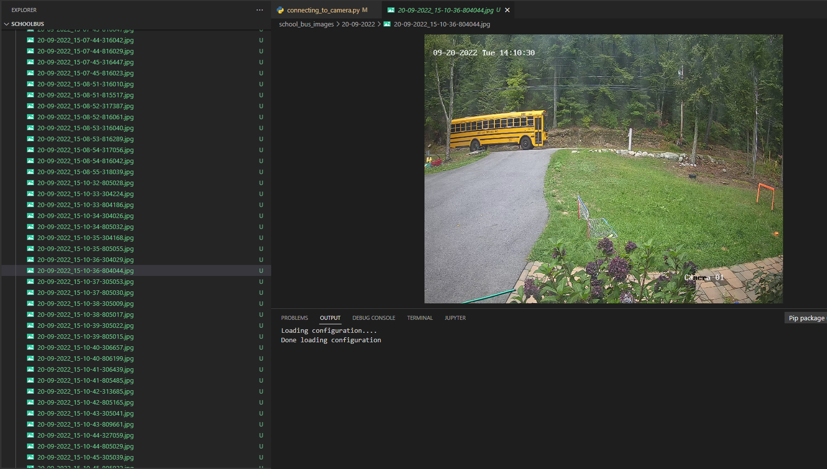

Data Collection:

These images will work great because they're of the actual scenery and object I'm looking to detect. Originally I had taken a video of the school bus pass my house on my phone. I then used a short script in R to turn that video into images. Live and learn, the frames from the actual camera are much more effective. There were many other things I learned during the data collection process as well. This is really my first time working with image data. I had tried using photos of buses from the internet, but this introduced orientations, colors and other things that I didn't need. My front yard will always look the same (with the exception of snow and being darker in the winter), so the buses from the internet didn't make sense for the project. If I was to extend this project to other use cases I absolutely might think about leveraging images from the internet or using more data augmentation. I made sure to include plenty of partial busses and images of the bus going both directions past my house.

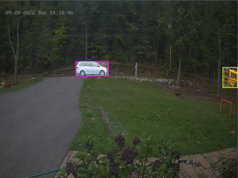
The model also detects cars and people quite well, but it was only trained on data that happened to be in front of my camera. I also annotated some bicycles, but that class isn't working well in my model at all.

I wish I had thought about how I planned on organizing my images from the beginning. Between using video from my phone, to leveraging images from the internet, different file formats being required for different algorithms (I started with yolov3 and then tried a classification algorithm before going with yolov5, they all required different file format and structure), I ended up with a lot of different data folders that I did not manage well. Then when I put the project down for the summer because school was out, when I came back in the fall I was really confused as to where my most recent images were. This is when I decided I was going to set up a Comet artifact to help manage my data, but we'll talk more about that in a future article.

Wonderful! We've talked about my considerations when getting images and hopefully your camera is now up and running. The next step is to annotate the images. I personally set up a free account in Roboflow, the UI was super intuitive (as you can see below) and I was able to annotate my images very quickly. You just click on the big "+ Create New Project" button, give the project a name and select "object detection" from the "Product Type" menu, on the next page select "upload" from the left nav and then you can upload your images.

Summary:

In this article we set ourselves up to begin a computer vision project. Although I’d love to keep this article going, I’m going to be breaking this project up into digestible chunks. We looked at the different libraries we’ll be using throughout the project, set up our camera, created images, and got ourselves set up to annotate all of those images. Next, we'll be talking about getting the data out of Roboflow, creating a data artifact in Comet, and training a yolov5 model. Since I'm chatting about Roboflow, the next article is actually going to be a guest blog on the Roboflow site. I'll make sure that all the articles are easy to navigate and find. After that we’ll choose the best model from the training runs by looking at the different experiments in Comet and use this to detect the bus live while watching the output live. Finally, we’ll be configuring how to send out text alerts using AWS. Lots of fun pieces in this project. It sounds like a lot, but I hope this feels like a project you’ll be able to do on your own! Stay tuned for the rest of the series. Click here to read the next article in the series.

9/12/22 9/12/22

Concatenating and Splitting Strings in R

Welcome! Here we're going to go through a couple examples of concatenating, subsetting and splitting strings in R. The motivation for this article is to show how simple working with strings can be with stringr. Working with strings was one of the areas that seemed intimidating and kept me from moving from Excel to R sooner, but many of the things I needed to do in Excel with strings are quite simple in R.

This article is really focusing on examples that I've experienced in Excel and how to do them in R. An example of when I've had to concatenate in the past is when someone handed me a dataset that included people's names and phone numbers, but they had not included a column with an id. I concatenated names and phone numbers to create a unique id for users. That's probably something you're not supposed to do (and I'd only recommend for an ad-hoc analysis without a ton of data), but it worked well enough for this particular use case. Using the "left" and "right" functions in Excel were also pretty common for me, and again, this is very easy to do in R. In this article we're going to cover:

Concatenating strings
Subsetting strings
Splitting strings

To do these string manipulations, we're going to be using the stringr and tidyr libraries. The cheat sheet for the stringr library can be found here. The tidyr cheat sheet can be found here. My friend Yujian Tang will be doing an almost similar article in python. You can find Yujian's article here.

Concatenate a string in r:

Concatenating is a fancy terms for just chaining things together. Being able to manipulate strings is one of the skills that made me feel more comfortable moving away from Excel and towards using code for my analyses. Here, we're just going to call in the stringr, dplyr, and tidyr libraries, create some data, and then concatenate that data. I've chosen to add the code here in a way that is easy to copy and paste, and then I've also added a screenshot of the output.

### install and call the stringr library
#install.packages("stringr")
#install.packages("dplyr")
#install.packages("tidyr")
library(stringr)
library(dplyr)
library(tidyr)  # for the separate function in splitting strings section

####  Create data
column1 <- c("Paul", "Kristen", "Susan", "Harold")
column2 <- c("Kehrer", "Kehrer", "Kehrer", "Kehrer")

##concatenate the columns
str_c(column1, column2)

Super simple, but also rarely what we're actually looking to achieve. Most of the time I'll need some other formatting, like a space between the names. This is super easy and intuitive to do. You're also able to put multiple concatenations together using the "collapse" parameter and specify the characters between those.

## Put a space between the names
str_c(column1, " ", column2)

###  If you were trying to make some weird sentence, I added apostrophes for the names:
str_c("We'll put the first name here: '", column1, "' and we'll put the second name here: '", column2,"'")

###  Using the collapse parameter, you're also able to specify any characters between the concatenations.  So column 1 and 2 will be concatenated, 
###  but each concatenation will be separated by commas

str_c(column1, " ", column2, collapse = ", ")

NAs by default are ignored in this case, but if you'd like them to be included you can leverage the "str_replace_na" function. This might be helpful if you're doing further string manipulation later on and don't want all your data to be consistent for future manipulations.

###  If you're dealing with NA's, you'll just need to add the "str_replace_na" function if you'd like it to be treated like your other data.
### Here is the default handling of NAs

column3 <- c("Software Engineer", "Data Scientist", "Student", NA)

str_c(column1, " - ", column3, ", ")

###  To make this work with the NA, just add "str_replace_na" to the relevant column

str_c(column1, " - ", str_replace_na(column3))

Subsetting a String in R:

Here, I was really focused on just sharing how to get the first couple elements or the last couple elements of a string. I remember in my Excel days that there would sometimes be a need to keep just the 5 characters on the right (or the left), especially if I received data where a couple columns had already been concatenated and now it needed to be undone. In R indexes start with "1", meaning the first object in a list is counted at "1" instead of "0". Most languages start with "0", including python. So here we go, looking at how you'll get the left and right characters from a string. First we'll get the original string returned, then we'll look at the right, then finally we'll do the same for the left.

### This will give me back the original string, because we're starting from the first letter and ending with the last letter
str_sub(column1, 1, -1)

### Here we'll get the 3 characters from the right.
### So this is similar to the "right" function in Excel.  
### We're telling the function to start at 3 characters from the end (because it's negative) and continue till the end of the string.
str_sub(column1, -3)

### The following would do the same, because the last element in the string is -1.
str_sub(column1, -3, -1)

###  Since the first input after the data is the "start" and the second is the "end", it's very easy to get any number of characters starting at the left of the string.
###  Here we're going from the first character to the third character.  So we'll have the first 3 characters of the string.
str_sub(column1, 1, 3)

Splitting A String in R:

When you have something like a column for the date that includes the full date, you might want to break that up into multiple columns; one for month, one for day, one for year, day of the week, etc. This was another task that I had previously done in Excel and now do in R. Any of these columns might be super useful in analysis, especially if you're doing time series modeling. For this we can use the separate function from tidyr (that we already loaded above). All we're doing here is passing the data to use and a vector of our desired column headings.

###  Create our data
dates <- c("Tuesday, 9/6/2022", "Wednesday, 9/7/2022", "Thursday, 9/8/2022")

###  Make this into a dataframe for ease of use
dates <- data.frame(dates)

### The separate function will create columns at each separator starting from the left.  If I only gave
### two column names I would be returned just the day of week and the month.
dates %>% separate(dates, c("day_of_week","month","day","year"))

And there you have it. These were a couple examples of working with strings I experienced as a wee analyst in Excel, but now would perform these tasks in R. Hope there is a person out there that needs to perform these tasks and happens to stumble upon this article. If you're looking to learn R, the best classes I've found are from Business Science. This (affiliate) link has a 15% off coupon attached. Although it's possible to buy the courses separately, this would bring you through using R for data science, you'll learn all the way through advanced shiny, and time series. The link to the Business Science courses is here. There is obviously so much more to working with strings than was explained here, but I wanted to just show a couple very clear and easy to read examples. Thanks for reading and happy analyzing.

8/10/22 8/10/22

Using Rename and Replace in Python To Clean Image Data

Over the years, I've made more silly mistakes than I can count when it comes to organizing my tabular data. At this point, I probably manage tabular data with my eyes closed. However, this is my first time really working with image data and I made a bunch of mistakes. That's what we're going to dive into in this article. Things like saving the annotations in the wrong file format when they were supposed to be .xml.

via GIPHY

For the person out there that has never played with image data for object detection, you have both the image file (I had jpeg) and an annotation file for each image that describes the bounding box of the object in the image and what the particular image is. I was using .xml for the notation files, another popular format is JSON.

I not only needed to change the file format to .xml, I had also made a couple other mistakes that I needed to fix in the annotation files. I thought that these little code snippets would be valuable to someone, I can't be the only person to make these mistakes. Hopefully this helps someone out there. The little scripts we're going to look at in this article are:

Changing the file path of the annotations
Changing "bus" to "school bus" in annotations, because I hadn't been consistent when labeling
Changing the names of images
Changing the file type to .xml

All of these above bullets basically make this a mini tutorial on for loops, replace, and rename in python.

The problem I'm solving

I just want to quickly provide some context, so it makes more sense why I'm talking about school buses. These data issues I'm fixing were through working on a computer vision project to detect the school bus driving by my home. My family is lucky because the school bus has to drive past my house and turn around before picking up my daughter at the end of the driveway. We've set up a text alert when the bus drives by, and it's the perfect amount of time to put our shoes on and head out the door. I came up with this project as a way to try out the CometML software that handles experiment tracking.

Changing the file path and making object names consistent

This first little snippet of code is going to loop through and change all of the annotation files. It'll open an annotation file, read that file, use the replace function twice to fix two different mistakes I made in the .xml file (storing it in the content variable), and then we're writing those changes to the file.

Since the level of this blog article is supposed to be very friendly, once you import "os", you can use os.getcwd() to get your current working directory. My file path is navigating to my data from the current working directory, this is called a relative file path. If you were to start your file path with "C:\Users\Kristen", etc. that's an "absolute" file path. An absolute file path will absolutely work here, however, relative file paths are nice because if the folder with your project ever moves an absolute path absolutely won't work anymore.

import os

###  Where the files live
files = os.listdir("datafolder/train/annotation/")

#print(files)

for file in files:
### In order to make multiple replacements, I save the output of Python's string replace() method in the same variable multiple times
    contents = open("datafolder/train/annotation/" + file,'r').read()
###  I was updating the annotation files to contain the correct file path with .xml inside the file, but you could replace anything
    contents = contents.replace("[content you need replaced]", 
    "[new content]")
### I had labeled some images with "bus" and some with "school bus", making them all consistent
    contents = contents.replace("school bus", "bus")
    write_file = open("datafolder/train/annotation/" + file,'w')
    write_file.write(contents)
    write_file.close()

Changing the names of images

Next up, I had created image datasets from video multiple times. I had written an article about how I created my image dataset from video in R here. I'll also be writing an article about how I did it in python, once I have that written I'll be sure to link it in this article.

If you're brand new to computer vision, the easiest way I found to have targeted image data for my model was to create the dataset myself. I did this by just taking a video of the bus driving by my house, then using a script to take frames from that video and turn it in to images.

Each time I created a new set of image data (I had converted multiple videos), the names of the images started with "image_00001". As I'm sure you know, this meant that I couldn't put all of my images in a single folder. Similar problem, still using the replace function, but we were using the function to change information inside a file before, now we're changing the name of the file itself. Let's dive in to changing the names of the image files.

Again, this is a simple for loop, and I'm just looping through each image in the directory, creating a new file name for the image using "replace", then renaming the whole file path plus image name so that our image is in the directory with the appropriate name. Rename is an operation on the file: "Change the file name from x to y". Replace is a string operation: "Replace any occurence of 'foo' in string X with 'bar'.

import os

dir = "datafolder/train/images/"

for file in os.listdir(dir):
    new_file = file.replace("image_0","bus")
###  now put the file path together with the name of the new image and rename the file to the new name.
    os.rename(dir + file, dir + new_file)

Changing the file type to .xml

My biggest faux pas was spending the time to manually label the images but saving them in the wrong file type. The documentation for labelImg was quite clear that they needed to be in Pascal VOC format, which is an .xml file. Since I had manually labeled the data, I wasn't looking to re-do any of my work there. Again, we're looping through each photo and using the rename function to rename the image

import os

path = 'datafolder/train/annotation/'
i = 0
for filename in os.listdir(path):
    os.rename(os.path.join(path,filename), os.path.join(path,'captured'+str(i)+'.xml'))
    i = i +1

Summary

If you're playing with computer vision, I highly suggest checking out the comet_ml library. With just a couple lines of code it'll store a snapshot of your dependencies, code and anything else you need for your model runs to be reproducible. This is an absolute life saver when you later run into a bug and you're not sure if it's a problem with your dependencies, etc. You'll also get a bunch of metrics and graphics to help you assess your model and compare it to other model runs right out of the box.

Hopefully you feel as though you're more comfortable using the rename and replace functions in python. I thought it was super fun to demonstrate using image data. There are so many more pieces to the computer vision project I'm working on and I can't wait to share them all.

8/3/22 8/3/22

An Analysis of The Loss Functions in Keras

Welcome to my friendly, non-rigorous analysis of the computer vision tutorials in keras. Keras is popular high-level API machine learning framework in python that was created by Google. Since I'm now working for CometML that has an integration with keras, I thought it was time to check keras out. This post is actually part of a three article series. My friend Yujian Tang and I are going to tag-team exploring keras together. Glad you're able to come on this journey with us.

This particular article is about the loss functions available in keras. To quickly define a loss function (sometimes called an error function), it is a measure of the difference between the actual values and the estimated values in your model. ML models use loss functions to help choose the model that is creating the best model fit for a given set of data (actual values are the most like the estimated values). The most well-known loss function would probably be the Mean Squared Error that we use in linear regression (MSE is used for many other applications, but linear regression is where most first see this function. It is also common to see RSME, that's just the square root of the MSE).

Here we're going to cover what loss functions were used to solve different problems in the keras computer vision tutorials. There were 68 computer vision examples, and 63 used loss functions (not all of the tutorials were for models). I was interested to see what types of problems were solved and which particular algorithms were used with the different loss functions. I decided that aggregating this data would give me a rough idea about what loss functions were commonly being used to solve the different problems. Although I'm well versed in certain machine learning algorithms for building models with structured data, I'm much newer to computer vision, so exploring the computer vision tutorials is interesting to me.

Things that I'm hoping to understand when it comes to the different loss functions available in keras:

Are they all being used?
Which functions are the real work horses?
Is it similar to what I've been using for structured data?

Let's start with the available loss functions. In keras, your options are:

The Different Groups of Keras Loss Functions

The losses are grouped into Probabilistic, Regression and Hinge. You're also able to define a custom loss function in keras and 9 of the 63 modeling examples in the tutorial had custom losses. We'll take a quick look at the custom losses as well. The difference between the different types of losses:

Probabilistic Losses - Will be used on classification problems where the ouput is between 0 and 1.

Regression Losses - When our predictions are going to be continuous.

Hinge Losses - Another set of losses for classification problems, but commonly used in support vector machines. Distance from the classification boundary is taken into account and you're penalized if the distance is not large enough.

This exercise was also a fantastic way to see the different types of applications of computer vision. Many of the tutorials I hadn't thought about that particular application. Hopefully it's eye-opening for you as well and you don't even have to go through the exercise of looking at each tutorial!

To have an understanding of the types of problems that were being solved in the tutorials, here's a rough list:

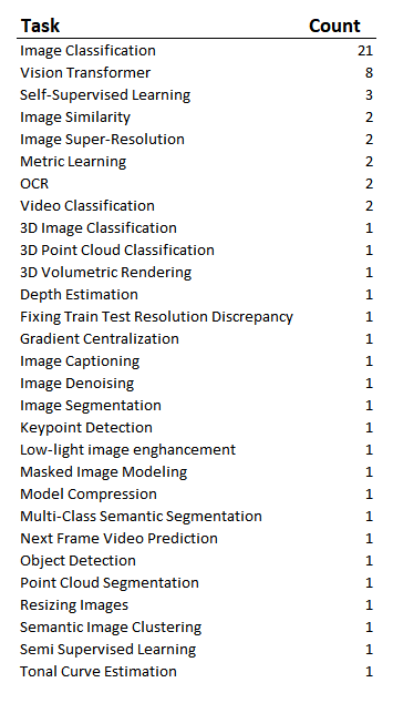
Image Classification Loss Functions

So of course, since Image classification was the most frequent type of problem in the tutorial, we're expecting to see many probabilistic losses. But which ones were they? The most obvious question is then "which loss functions are being used in those image classification problems?"

We see that the sparse categorical crossentropy loss (also called softmax loss) was the most common. Both sparse categorical crossentropy and categorical cross entropy use the same loss function. If your output variable is one-hot encoded you'd use categorical cross entropy, if your output variable is integers and they're class indices, you'd use the sparse function. Binary crossentropy is used when you only have one classifier . In the function below, "n" is the number of classes, and in the case of binary cross entropy, the number of classes will be 2 because in binary classification problems you only have 2 potential outputs (classes), the output can be 0 or 1.

Keras Custom Loss Functions

One takeaway that I also noticed is that there weren't any scenarios here where a custom defined loss was used for the image classification problems. All the classification problems used one of those 3 loss functions. For the 14% of tutorials that used a custom defined function, what type of problem were they trying to solve? (These are two separate lists, you can't read left to right).

Regression Loss Functions

Now I was also interested to see which algorithms were used most frequently in the tutorial for regression problems. There were only 6 regression problems, so the sample is quite small.

It was interesting that only two of the losses were used. We did not see mean absolute percentage error, mean squared logarithmic error, cosine similarity, huber, or log-cosh. It feels good to see losses that I'm most familiar with being used in these problems, this feels so much more approachable. The MSE is squared, so it will penalize large differences between the actual and estimated more than the MAE. So if "how much" your estimate is off by isn't a big concern, you might go with MAE, if the size of the error matters, go with MSE.

Implementing Keras Loss Functions

If you're just getting started in keras, building a model looks a little different. Defining the actual loss function itself is straight forward, but we can chat about the couple lines that precede defining the loss function in the tutorial (This code is taken straight from the tutorial). In keras, there are two ways to build models, either sequential or functional. Here we're building a sequential model. The sequential model API allows you to create a deep learning model where the sequential class is created, and then you add layers to it. In the keras.sequentional() function there are the optional arguments "layers" and "name", but instead we're adding the layers piecewise.

The first model.add line that we're adding is initializing the kernel. "kernel_initializer" is defining the statistical distribution of the starting weights for your model. In this example the weights are uniformly distributed. This is a single hidden layer model. The loss function is going to be passed during the compile stage. Here the optimizer being used is adam, if you want to read more about optimizers in keras, check out Yujian's article here.

from tensorflow import keras
from tensorflow.keras import layers

model = keras.Sequential()
model.add(layers.Dense(64, kernel_initializer='uniform', input_shape=(10,)))
model.add(layers.Activation('softmax'))

loss_fn = keras.losses.SparseCategoricalCrossentropy()
model.compile(loss=loss_fn, optimizer='adam')

Summary

I honestly feel better after taking a look at these computer vision tutorials. Although there was plenty of custom loss functions that I wasn't familiar with, the majority of the use cases were friendly loss functions that I was already familiar with. I also feel like I'll feel a little more confident being able to choose a loss function for computer vision problems in the future. Sometimes I can feel like things are going to be super fancy or complicated, like when "big data" was first becoming a popular buzzword, but then when I take a look myself it's less scary than I thought. If you felt like this was helpful, be sure to let me know. I'm very easily findable on LinkedIn and might make more similar articles if people find this type of non-rigorous analysis interesting.

And of course, if you're building ML models and want to be able to very easily track, compare, make your runs reproducible, I highly suggest you check out the CometML library in python or R :)

Kristen Kehrer 5/16/22 Kristen Kehrer 5/16/22

How To Create A Computer Vision Dataset From Video in R

I wanted to write a quick article about creating image datasets from video for computer vision. Here we'll be taking a video that I took on my phone and create training and validation datasets from the video in R. My hope is that someone who is new to playing with computer vision stumbles on this article and that I'm able to save this person some time and extra googling. I get giddy when I find a blog article that does exactly what I want and is simple to understand, I'm just trying to pay it forward. The project I'm working on is written in python, so unfortunately I won't be helping you go end-to-end here, unless you're looking to continue in python. To create the dataset, I used the av library in R. The av library in R makes it crazy simple to split a video you take on your phone into a bunch of images and save them in a folder. Once you have that, you'll of course need to take a random sample of files to place in a training dataset folder you'll create, and then you'll want to place the remaining images in a validation dataset folder. Easy peasy. I did not attempt to do anything fancy, I'm hoping this will feel very friendly.

######################################################################
###  Creating a folder with a bunch of images from video

###  The only library we need for this:
library("av")

### The path where you've saved the video and where you want your images
video_path = "[path to movie]/[your movie].MOV"
path = "[path to new folder]"

###    set your working directory to be where the files are stored
setwd(path)

###  Function that will give you all your frames in a folder
###  First we're just dumping all of the images into a single folder, we'll split test and 
###  validation afterwards
av_video_images(video = video_path, destdir = path, format = "jpg", fps = NULL)

###    How many images are in that folder?  Just checking for context
length(list.files())

Now we have a folder with all of our images. Next we're going to take a random sample of 70% of the images for our training set. Then we'll move those files to a training folder. Get excited to move some files around!

via GIPHY

####################################################################################
#### Now creating the testing and validation sets


###    Now Take a sample of 70% of the images for the training set, we do not want with replacement 
images_training <- sample(list.files(),length(list.files())*.7, replace = FALSE)


####   Create training and validation folders so we have a place to store our photos
####   If the training folder does not exist, create training folder (with dir.create), else tell me it already exists
ifelse(!dir.exists("training"), dir.create("training"), "Folder exists already")
ifelse(!dir.exists("validation"), dir.create("validation"), "Folder exists already")


###   Place training images in the training folder
###   Here we are going to loop through each image and copy the folder from the old path 
###   to the new path (in our training folder)
for (image in images_training) {
     new_place <- file.path(path, "training",image)  ### pointing to the new training file path
     old_place <- file.path(path,image)
     file.copy(from = old_place, to = new_place)
}

Next we're going to remove the training images from their original folder, so that all we'll have left in the original folder is the validation images. Just gonna do a little cleanup here. To do this, we'll simply loop through each image, and in each iteration of the loop, we're removing an image.

via GIPHY

for (image in images_training) {
  file.remove(path, image)
  }

###  Double check that the length looks right
length(list.files())


###    Put remaining image files in validation folder
images_validation <- list.files()

for (image in images_validation) {
  new_place <- file.path(path, "validation", image)
  old_place <- file.path(path,image)
  file.copy(from = old_place, to = new_place)
}

####  Remove the validation images from the old folder (this is just cleanup)
####  For is image in the remaining list of files, remove the image.
for (image in list.files()) {
  file.remove(path, image)
}

Now you're all set up to start using these images from a video you've taken yourself! If you're playing with computer vision, I highly suggest checking out the cometr library. With just a couple lines of code it'll store a snapshot of your dependencies, code and anything else you need for your model to be reproducible. This is an absolute life saver when you later run into a bug and you're not sure if it's a problem with your dependencies, etc. cometr makes it so you'll be able to just check on your last successful run, easily compare with the current code, see what the discrepancy was, and continue on your merry way. If the libraries for computer vision that you're using integrate with comet, then you'll also get a bunch of metrics and graphics to help you assess your model right out of the box.

From here, you'll want to create bounding boxes for the images. The easiest way I've found to do this is leveraging the labelImg library in python. You just pip install the labelImg package and then run labelImg in python and a GUI pops up for creating the bounding boxes. It really can't get much easier than that. If you happen upon a great way to label the images that doesn't involve python, please let me know. I would love to suggest something non-python here because this is obviously not a python article. Thanks for reading! Hope you have the easiest time turning your video into an image dataset for training and validation, and may your object detection models detect all the things.

Originally published athttps://heartbeat.comet-ml.com/ on June 2, 2022.

9/10/19 9/10/19

Choosing the Correct Statistic for Your Hypothesis Test

I fondly remember learning how to use countless statistics for evaluating hypothesis tests while getting my Master's degree. However, it was much more difficult to learn which method to call upon when faced with evaluating a real hypothesis test out in the world. I've previously written about scoping hypothesis tests with stakeholders, and test design and considerations for running hypothesis tests. To continue the saga, and complete the Hypothesis Testing trilogy (for now at least), I'd like to discuss a method for determining the best test statistic to use when evaluating a hypothesis test. I'll also take you through a code example where I compare the results of using 2 different statistics to evaluate data from a hypothetical ecommerce website.

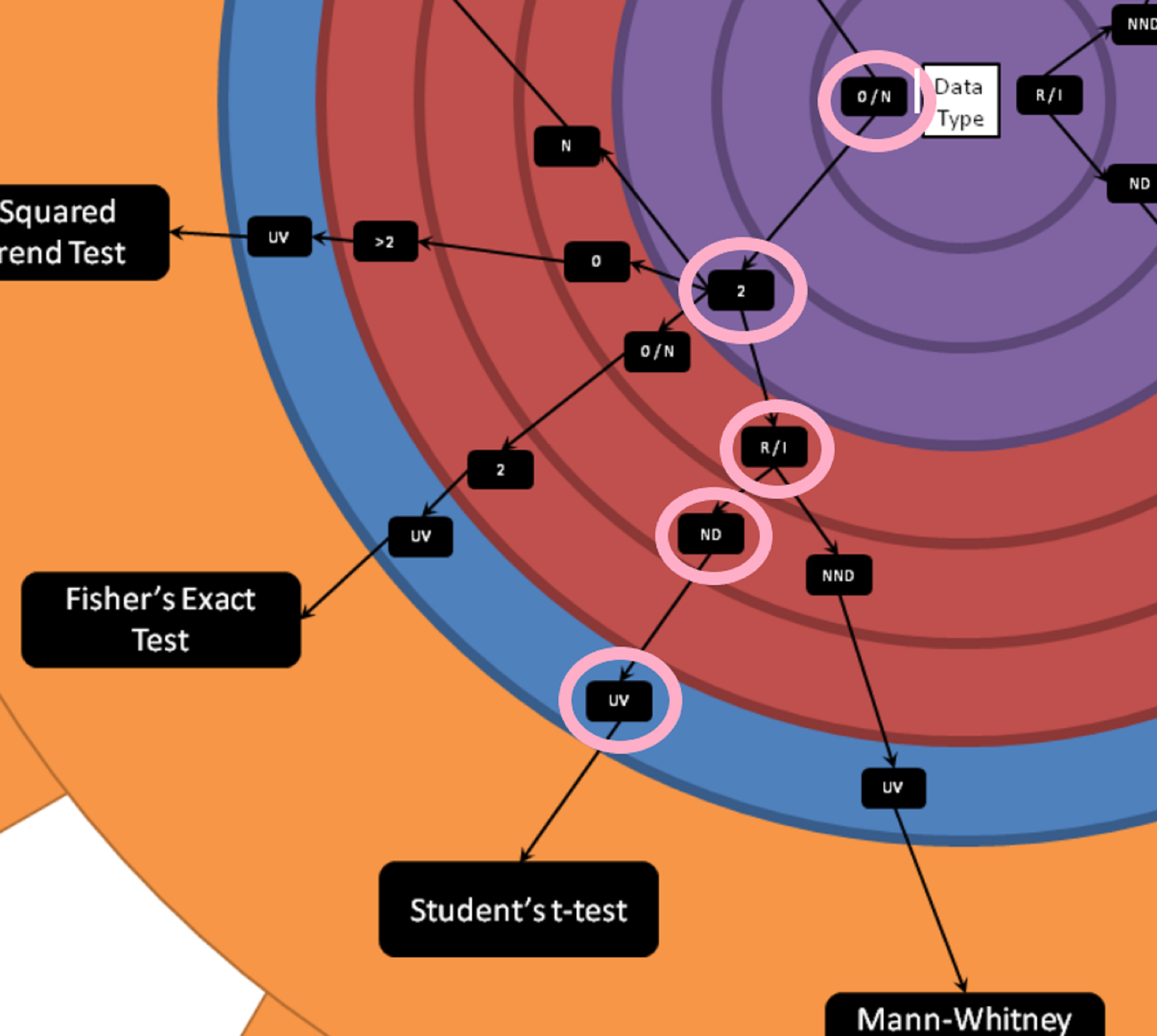
Lee Baker's Hypothesis Testing Wheel

Lee Baker from Chi2Innovations has developed a wonderful visual tool which, frankly, I wish I had when I was first learning about all the different types of test statistics. He calls it the "Hypothesis Testing Wheel", and it provides a repeatable set of questions whose answers will lead you to the best single choice for your situation. You can get a copy of this wheel in your inbox by giving your email at this link: I want a printout

Below is a picture of the wheel:

How to use the wheel

To determine which test statistic to use, you begin in the center of the large wheel and assess which data type you'll be testing.

Is the data in your test test:

Interval - Continuous, and the difference between two measures is meaningful.
Ratio - All the properties of an interval variable, variables like height or weight, but must also have a clear definition of 0.0 (and that definition has to be None).
Ordinal - Categorical, and ordered.
Nominal - Categorical, order doesn't matter
Mixed (multiple types of the above)

From the center you'll move outwards. And for continuous variables you'll need to determine next whether your variables are roughly normally distributed or not. In the example below we'll be looking at a hypothetical test of conversion on a website. Conversion rate is a proportion, but the individuals rows of data is categorical. Either a customer converts or does not convert. The mean of the proportion of customers who convert on a website is roughly normally distributed thanks to the Central Limit Theorem. In the case of categorical variables you're asked about the number of classes in your variable. You'll also need to determine whether your analysis is univariate or multivariate. In the hypothetical conversion example we're discussing, this is a univariate test.

Example using the wheel

In our example we have a hypothetical test on a website. Each visitor can either convert or not convert. This is ordinal data, as converting is set to 1, and converting is considered more valuable than not converting. We also know that we have 2 categories (converted or not converted). The outcome we're measure is the total proportion of converted customers, the data type for that would be ratio. We can assume rough normality due to the central limit theorem, and this is a univariate test. Therefore, we determine that we can use Student's t-test to evaluate our hypothetical test.

Example Analyzing in R

You're able to download the data and follow along here: hypothesis_test

This is a hypothetical website test. The dataset contains the following data:

test_assignment: Whether you were assigned to test or control
Conv: Where you're assigned to either the test or control group (test = 1, control = 0) and you either converted or did not convert (converted = 1)
Quantity: How much of the item you purchased (we're assuming only a single product is for sale, but you can buy multiple of that product)
Sales: The total price of the customers purchase
Cost_of_good: How much it costs to create the product

We'll call in the data and do some filtering to get the data ready for analysis. Then we'll perform a Student's t-test, the Chi-Sq test of Proportions, and compare the results.

Code

library(stats)  ##   For student's t-test
library(tidyverse)  ##   For data manipulation

# Set working directory, please update with your own file path:
# Remember backslashes need to be changed to forward slashes
setwd("[your path here]")

# reading in the data
web_test <- read.csv("hypothesis_test.csv")

# Looking at the structure of the data
str(web_test)

# Changing test_assignment to a factor variable.
# This is  a factor and not truly valued at 1 or 0
web_test$test_assignment <- as.factor(web_test$test_assignment)

# Remmoving those who saw both the test and control experience 
# Or were duplicates in our data and saving as a new dataset.
web_test_no_dupes <- web_test %>%
  filter(!duplicated(customer_id))



# Creating a set with just test and just control so that the data is separated
test <- web_test_no_dupes %>%
  filter(test_assignment == 1)

control <- web_test_no_dupes %>%
  filter(test_assignment == 0)


###
# Student's t-test (assumes equal variance, otherwise it's Welch's t-test)
# here we pass the vectors of the 1's and 0's
test<- t.test(test$Conv, control$Conv, var.equal = TRUE)


###
# Chi-Squared Test of Equality of Proportions
# here I'm passing the total number of conversions in each group and the sample size in 
# both test and control.  

# creating a vector with numerator and denominator for the test
numerator <- c(sum(test$Conv), sum(control$Conv))
denominator <- c(length(test$Conv), length(control$Conv))

# Perforoming the Chi-Sq test below
# correct = FALSE is saying that I will not be using a continuity correction in this example
# setting it equal to TRUE would give us a slightly more conservative estimate.
chisq <- prop.test(numerator, denominator, correct = FALSE)

Output from the two tests

You'll notice that the confidence intervals are almost exactly the same. Both tests were statistically significant, but that was expected anyways because of the large difference between proportions. However, the most important thing when analyzing hypothesis tests is that you're consistent across your organization. You certainly do not want one person doing the analysis and returning a different result than if someone else had conducted the analysis.

If your R skills could use some work and you'd like to become truly proficient, I recommend the following R courses.

Summary:

I found Lee's cheat sheet quite handy (and I hadn't seen something like it previously). He also has a great blog where he focuses heavily on statistics. I find that when people are trying to learn stats, they're always looking for more resources to read up on the material. Lee's blog is a fantastic resource for free e-books, probability, stats, and data cleaning. A link to Lee's blog is here.

Thanks for reading! I'm happy to have added more content around hypothesis testing on my blog. If there is something you'd like me to dive into deeper, don't hesitate to leave a comment and ask. Happy hypothesis testing, see you soon :)

10/21/18 10/21/18

Life Changing Moments of DataScienceGO 2018

DataScienceGO is truly a unique conference. Justin Fortier summed up part of the ambiance when replying to Sarah Nooravi's LinkedIn post.And although I enjoy a good dance party (more than most), there were a number of reasons why this conference (in particular) was so memorable.

Community
Yoga + Dancing + Music + Fantastic Energy
Thought provoking keynotes (saving the most life changing for last)

Community:In Kirill's keynotes he mentioned that "community is king". I've always truly subscribed to this thought, but DataScienceGO brought this to life. I met amazing people, some people that I had been building relationships for months online but hadn't yet had the opportunity to meet in person, some people I connected with that I had never heard of. EVERYONE was friendly. I mean it, I didn't encounter a single person that was not friendly. I don't want to speak for others, but I got the sense that people had an easier time meeting new people than what I have seen at previous conferences. It really was a community feeling. Lots of pictures, tons of laughs, and plenty of nerdy conversation to be had.If you're new to data science but have been self conscious about being active in the community, I urge you to put yourself out there. You'll be pleasantly surprised.Yoga + Dancing + Music + Fantastic EnergyBoth Saturday and Sunday morning I attended yoga at 7am. To be fully transparent, I have a 4 year old and a 1 year old at home. I thought I was going to use this weekend as an opportunity to sleep a bit. I went home more tired than I had arrived. Positive, energized, and full of gratitude, but exhausted.Have you ever participated in morning yoga with 20-30 data scientists? If you haven't, I highly recommend it.It was an incredible way to start to the day, Jacqueline Jai brought the perfect mix of yoga and humor for a group of data scientists. After yoga each morning you'd go to the opening keynote of the day. This would start off with dance music, lights, sometimes the fog machine, and a bunch of dancing data scientists. My kind of party.The energized start mixed with the message of community really set the pace for a memorable experience.Thought provoking keynotes Ben Taylor spoke about "Leaving an AI Legacy", Pablos Holman spoke about actual inventions that are saving human lives, and Tarry Singh showed the overwhelming (and exciting) breadth of models and applications in deep learning. Since the conference I have taken a step back and have been thinking about where my career will go from here. In addition, Kirill encouraged us to think of a goal and to start taking small actions towards that goal starting today.I haven't nailed down yet how I will have a greater impact, but I have some ideas (and I've started taking action). It may be in the form of becoming an adjunct professor to educate the next wave of future mathematicians and data scientists. Or I hope to have the opportunity to participate in research that will aid in helping to solve some of the world's problems and make someone's life better.I started thinking about my impact (or using modeling for the forces of good) a couple weeks ago when I was talking with Cathy O'Neil for the book I'm writing with Kate Strachnyi "Mothers of Data Science". Cathy is pretty great at making you think about what you're doing with your life, and this could be it's own blog article. But attending DSGO was the icing on the cake in terms of forcing me to consider the impact I'm making.Basically, the take away that I'm trying to express is that this conference pushed me to think about what I'm currently doing, and to think about what I can do in the future to help others. Community is king in more ways than one.ClosingI honestly left the conference with a couple tears. Happy tears, probably provoked a bit by being so overtired. There were so many amazing speakers in addition to the keynotes. I particularly enjoyed being on the Women's panel with Gabriela de Queiroz, Sarah Nooravi, Page Piccinini, and Paige Bailey talking about our real life experiences as data scientists in a male dominated field and about the need for diversity in business in general. I love being able to connect with other women who share a similar bond and passion.I was incredibly humbled to have the opportunity to speak at this conference and also cheer for the talks of some of my friends: Rico Meinl, Randy Lao, Tarry Singh, Matt Dancho and other fantastic speakers. I spoke about how to effectively present your model output to stakeholders, similar to the information that I covered in this blog article: Effective Data Science Presentations This article is obviously an over simplification of all of the awesomeness that happened during the weekend. But if you missed the conference, I hope this motivates you to attend next year so that we can meet. And I urge you to watch the recordings and reflect on the AI legacy you want to leave behind.I haven't seen the link to the recordings from DataScienceGo yet, but when I find them I'll be sure to link here.

10/1/18 10/1/18

Setting Your Hypothesis Test Up For Success

Setting up your hypothesis test for success as a data scientist is critical. I want to go deep with you on exactly how I work with stakeholders ahead of launching a test. This step is crucial to make sure that once a test is done running, we'll actually be able to analyze it. This includes:

A well defined hypothesis
A solid test design
Knowing your sample size
Understanding potential conflicts
Population criteria (who are we testing)
Test duration (it's like the cousin of sample size)
Success metrics
Decisions that will be made based on results

This is obviously a lot of information. Before we jump in, here is how I keep it all organized:I recently created a google doc at work so that stakeholders and analytics could align on all the information to fully scope a test upfront. This also gives you (the analyst/data scientist) a bit of an insurance policy. It's possible the business decides to go with a design or a sample size that wasn't your recommendation. If things end up working out less than stellar (not enough data, design that is basically impossible to analyze), you have your original suggestions documented.In my previous article I wrote:

"Sit down with marketing and other stakeholders before the launch of the A/B test to understand the business implications, what they’re hoping to learn, who they’re testing, and how they’re testing. In my experience, everyone is set up for success when you’re viewed as a thought partner in helping to construct the test design, and have agreed upon the scope of the analysis ahead of launch."

Well, this is literally what I'm talking about:This document was born of things that we often see in industry:HypothesisI've seen scenarios that look like "we're going to make this change, and then we'd like you to read out on the results". So, your hypothesis is what? You're going to make this change, and what do you expect to happen? Why are we doing this? A hypothesis clearly states the change that is being made, the impact you expect it to have, and why you think it will have that impact. It's not an open-ended statement. You are testing a measurable response to a change. It's ok to be a stickler, this is your foundation.Test DesignThe test design needs to be solid, so you'll want to have an understanding of exactly what change is being made between test and control. If you're approached by a stakeholder with a design that won't allow you to accurately measure criteria, you'll want to coach them on how they could design the test more effectively to read out on the results. I cover test design a bit in my article here.Sample SizeYou need to understand the sample size ahead of launch, and your expected effect size. If you run with a small sample and need an unreasonable effect size for it to be significant, it's most likely not worth running. Time to rethink your sample and your design. Sarah Nooravi recently wrote a great article on determining sample size for a test. You can find Sarah's article here.

An example might be that you want to test the effect of offering a service credit to select customers. You have a certain budget worth of credits you're allowed to give out. So you're hoping you can have 1,500 in test and 1,500 in control (this is small). The test experience sees the service along with a coupon, and the control experience sees content advertising the service but does not see any mention of the credit. If the average purchase rate is 13.3% you would need a 2.6 point increase (15.9%) in the control to see significance at 0.95 confidence. This is a large effect size that we probably won't achieve (unless the credit is AMAZING). It's good to know these things upfront so that you can make changes (for instance, reduce the amount of the credit to allow for additional sample size, ask for extra budget, etc).

Potential Conflicts:It's possible that 2 different groups in your organization could be running tests at the same time that conflict with each other, resulting in data that is junk for potentially both cases. (I actually used to run a "testing governance" meeting at my previous job to proactively identify these cases, this might be something you want to consider).

An example of a conflict might be that the acquisition team is running an ad in Google advertising 500 business cards for $10. But if at the same time this test was running another team was running a pricing test on the business card product page that doesn't respect the ad that is driving traffic, the acquisition team's test is not getting the experience they thought they were! Customers will see a different price than what is advertised, and this has negative implications all around.
It is so important in a large analytics organization to be collaborating across teams and have an understanding of the tests in flight and how they could impact your test.

Population criteria: Obviously you want to target the correct people. But often I've seen criteria so specific that the results of the test need to be caveated with "These results are not representative of our customer base, this effect is for people who [[lists criteria here]]." If your test targeted super performers, you know that it doesn't apply to everyone in the base, but you want to make sure it is spelled out or doesn't get miscommunicated to a more broad audience.

Test duration: This is often directly related to sample size. (see Sarah's article) You'll want to estimate how long you'll need to run the test to achieve the required sample size. Maybe you're randomly sampling from the base and already have sufficient population to choose from. But often we're testing an experience for new customers, or we're testing a change on the website and we need to wait for traffic to visit the site and view the change. If it's going to take 6 months of running to get the required sample size, you probably want to rethink your population criteria or what you're testing. And better to know that upfront.

Success Metrics: This is an important one to talk through. If you've been running tests previously, I'm sure you've had stakeholders ask you for the kitchen sink in terms of analysis.If your hypothesis is that a message about a new feature on the website will drive people to go see that feature; it is reasonable to check how many people visited that page and whether or not people downloaded/used that feature. This would probably be too benign to cause cancellations, or effect upsell/cross-sell metrics, so make sure you're clear about what the analysis will and will not include. And try not to make a mountain out of a molehill unless you're testing something that is a dramatic change and has large implications for the business.

Decisions! Getting agreement ahead of time on what decisions will be made based on the results of the test is imperative.Have you ever been in a situation where the business tests something, it's not significant, and then they roll it out anyways? Well then that really didn't need to be a test, they could have just rolled it out. There are endless opportunities for tests that will guide the direction of the business, don't get caught up in a test that isn't actually a test.

Conclusion: Of course, each of these areas could have been explained in much more depth. But the main point is that there are a number of items that you want to have a discussion about before a test launches. Especially if you're on the hook for doing the analysis, you want to have the complete picture and context so that you can analyze the test appropriately.I hope this helps you to be more collaborative with your business partners and potentially be more "proactive" rather than "reactive".

No one has any fun when you run a test and then later find out it should have been scoped differently. Adding a little extra work and clarification upfront can save you some heartache later on. Consider creating a document like the one I have pictured above for scoping your future tests, and you'll have a full understanding of the goals and implications of your next test ahead of launch. :)