Choosing the Correct Statistic for Your Hypothesis Test

I fondly remember learning how to use countless statistics for evaluating hypothesis tests while getting my Master's degree. However, it was much more difficult to learn which method to call upon when faced with evaluating a real hypothesis test out in the world. I've previously written about scoping hypothesis tests with stakeholders, and test design and considerations for running hypothesis tests. To continue the saga, and complete the Hypothesis Testing trilogy (for now at least), I'd like to discuss a method for determining the best test statistic to use when evaluating a hypothesis test. I'll also take you through a code example where I compare the results of using 2 different statistics to evaluate data from a hypothetical ecommerce website.

Lee Baker's Hypothesis Testing Wheel

Lee Baker from Chi2Innovations has developed a wonderful visual tool which, frankly, I wish I had when I was first learning about all the different types of test statistics. He calls it the "Hypothesis Testing Wheel", and it provides a repeatable set of questions whose answers will lead you to the best single choice for your situation. You can get a copy of this wheel in your inbox by giving your email at this link: I want a printout

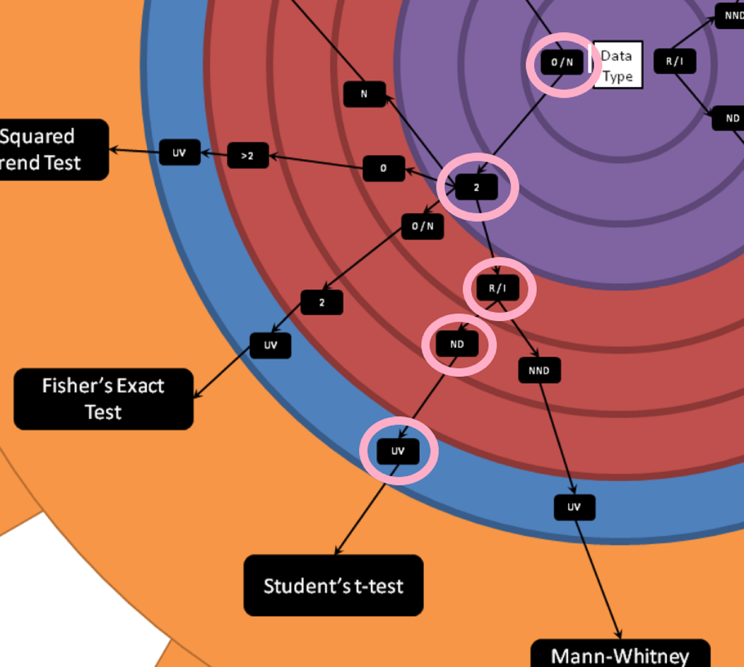
Below is a picture of the wheel:

How to use the wheel

To determine which test statistic to use, you begin in the center of the large wheel and assess which data type you'll be testing.

Is the data in your test test:

Interval - Continuous, and the difference between two measures is meaningful.
Ratio - All the properties of an interval variable, variables like height or weight, but must also have a clear definition of 0.0 (and that definition has to be None).
Ordinal - Categorical, and ordered.
Nominal - Categorical, order doesn't matter
Mixed (multiple types of the above)

From the center you'll move outwards. And for continuous variables you'll need to determine next whether your variables are roughly normally distributed or not. In the example below we'll be looking at a hypothetical test of conversion on a website. Conversion rate is a proportion, but the individuals rows of data is categorical. Either a customer converts or does not convert. The mean of the proportion of customers who convert on a website is roughly normally distributed thanks to the Central Limit Theorem. In the case of categorical variables you're asked about the number of classes in your variable. You'll also need to determine whether your analysis is univariate or multivariate. In the hypothetical conversion example we're discussing, this is a univariate test.

Example using the wheel

In our example we have a hypothetical test on a website. Each visitor can either convert or not convert. This is ordinal data, as converting is set to 1, and converting is considered more valuable than not converting. We also know that we have 2 categories (converted or not converted). The outcome we're measure is the total proportion of converted customers, the data type for that would be ratio. We can assume rough normality due to the central limit theorem, and this is a univariate test. Therefore, we determine that we can use Student's t-test to evaluate our hypothetical test.

Example Analyzing in R

You're able to download the data and follow along here: hypothesis_test

This is a hypothetical website test. The dataset contains the following data:

test_assignment: Whether you were assigned to test or control
Conv: Where you're assigned to either the test or control group (test = 1, control = 0) and you either converted or did not convert (converted = 1)
Quantity: How much of the item you purchased (we're assuming only a single product is for sale, but you can buy multiple of that product)
Sales: The total price of the customers purchase
Cost_of_good: How much it costs to create the product

We'll call in the data and do some filtering to get the data ready for analysis. Then we'll perform a Student's t-test, the Chi-Sq test of Proportions, and compare the results.

Code

library(stats)  ##   For student's t-test
library(tidyverse)  ##   For data manipulation

# Set working directory, please update with your own file path:
# Remember backslashes need to be changed to forward slashes
setwd("[your path here]")

# reading in the data
web_test <- read.csv("hypothesis_test.csv")

# Looking at the structure of the data
str(web_test)

# Changing test_assignment to a factor variable.
# This is  a factor and not truly valued at 1 or 0
web_test$test_assignment <- as.factor(web_test$test_assignment)

# Remmoving those who saw both the test and control experience 
# Or were duplicates in our data and saving as a new dataset.
web_test_no_dupes <- web_test %>%
  filter(!duplicated(customer_id))



# Creating a set with just test and just control so that the data is separated
test <- web_test_no_dupes %>%
  filter(test_assignment == 1)

control <- web_test_no_dupes %>%
  filter(test_assignment == 0)


###
# Student's t-test (assumes equal variance, otherwise it's Welch's t-test)
# here we pass the vectors of the 1's and 0's
test<- t.test(test$Conv, control$Conv, var.equal = TRUE)


###
# Chi-Squared Test of Equality of Proportions
# here I'm passing the total number of conversions in each group and the sample size in 
# both test and control.  

# creating a vector with numerator and denominator for the test
numerator <- c(sum(test$Conv), sum(control$Conv))
denominator <- c(length(test$Conv), length(control$Conv))

# Perforoming the Chi-Sq test below
# correct = FALSE is saying that I will not be using a continuity correction in this example
# setting it equal to TRUE would give us a slightly more conservative estimate.
chisq <- prop.test(numerator, denominator, correct = FALSE)

Output from the two tests

You'll notice that the confidence intervals are almost exactly the same. Both tests were statistically significant, but that was expected anyways because of the large difference between proportions. However, the most important thing when analyzing hypothesis tests is that you're consistent across your organization. You certainly do not want one person doing the analysis and returning a different result than if someone else had conducted the analysis.

If your R skills could use some work and you'd like to become truly proficient, I recommend the following R courses.

Summary:

I found Lee's cheat sheet quite handy (and I hadn't seen something like it previously). He also has a great blog where he focuses heavily on statistics. I find that when people are trying to learn stats, they're always looking for more resources to read up on the material. Lee's blog is a fantastic resource for free e-books, probability, stats, and data cleaning. A link to Lee's blog is here.

Thanks for reading! I'm happy to have added more content around hypothesis testing on my blog. If there is something you'd like me to dive into deeper, don't hesitate to leave a comment and ask. Happy hypothesis testing, see you soon :)